In this post, we will review the paper Morphing and Sampling Network for Dense Point Cloud Completion presented by Liu et al. at the AAAI 2020 in New York. We will take a quick look at the motivation and previous approaches on point cloud completion and then dive into the network architecture and review the experiments conducted on the network. To close off I present a conclusion and my view on the paper.

The code for this paper is available under https://github.com/Colin97/MSN-Point-Cloud-Completion.

Motivation

The eyes into the world of an autonomous vehicle are the sensors installed on the vehicle. In order to understand the environment in which the vehicle is driving and to make informed decisions about potential paths of actions it’s important to have reliable and complete sensor data about the scene. Such 3D data is commonly collected with Lidar sensors which capture a scene as a set of distinct points, referred to as a point cloud. Even though Lidar produces high fidelity scans, there are two main factors which can lower the quality of the 3D scans.

First, scans are often obtained from a single view angle. This means that any part of an object which is occluded by itself or by other objects in the scene will be missing in the obtained point cloud.

Second, the capacity of the sensor limits the fidelity of the scan. While objects in the foreground of the scene will be represented by many points, objects in the back may only be represented by a handful of points.

You can imagine that any tasks that we want to perform on the point cloud, such as semantic segmentation or object classification are very difficult if parts of the data are missing. Therefore, we could greatly improve the performance of these subsequent tasks by first completing objects in the points cloud. This is the idea behind point cloud completion: We get as input an incomplete point cloud and are assigned the task of completing the shapes of certain objects in the point cloud. Some examples of partial input shapes and complete shapes can be seen in the image below.

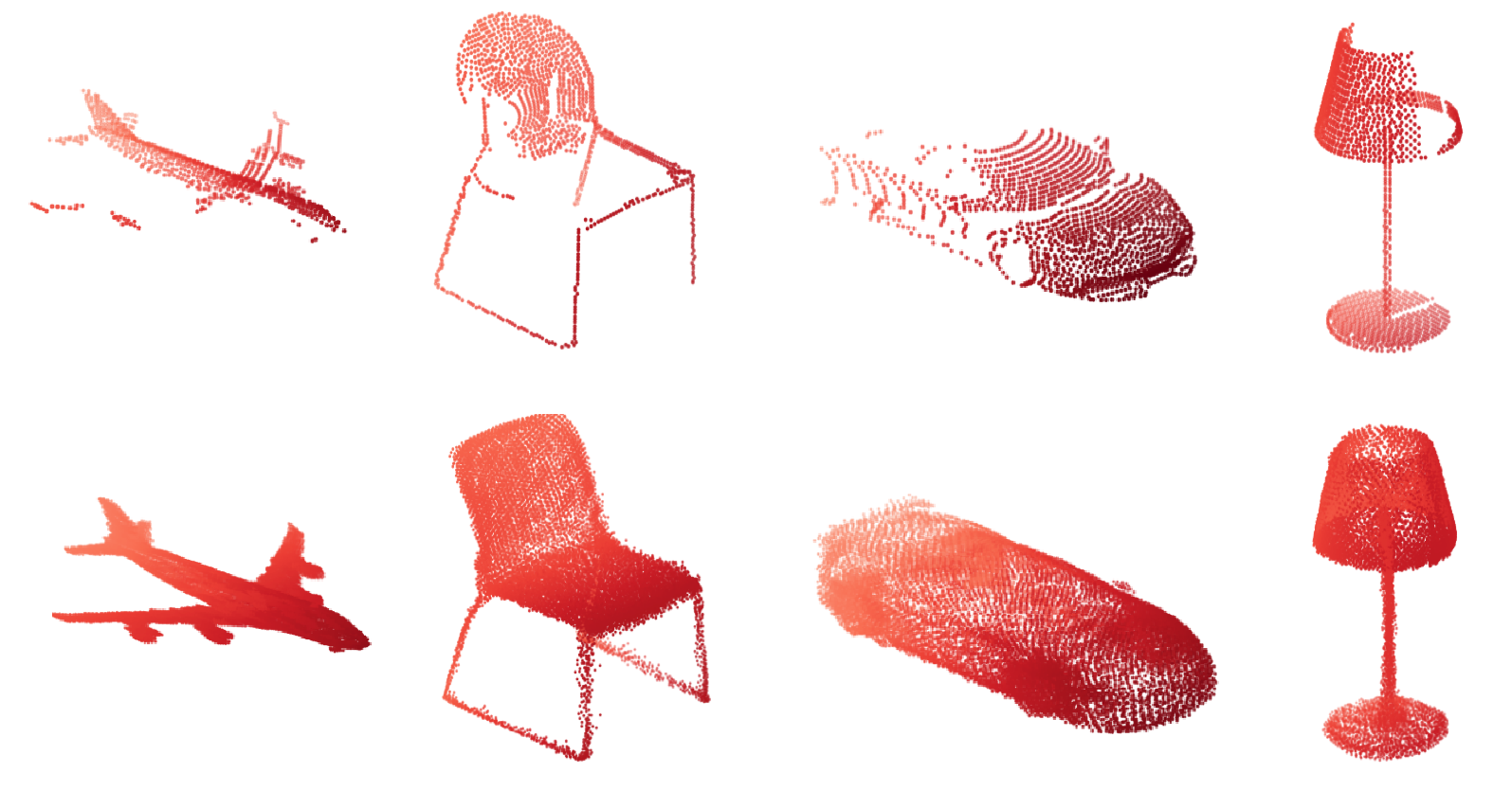
3D Shape Completion

In this section, I will present some of the methods that can be used to complete a partial 3D shape. These methods can be partitioned into three main avenues: Geometry-based, example-base and learning-based.

Geometry-based

Geometry-based approaches aim to complete parts of the shape by extrapolating from existing parts in the input, either by interpolation or using assumptions about symmetry in the object. Interpolation fails on large-scale incompleteness and symmetry is not given for all objects so this approach has some clear drawbacks.

Example-based

The second approach involves example-based methods. Here, we have a database of existing shapes which we then deform and assemble to form the complete shape of the object. You can imagine that this method fails for unseen shapes which are not present in the shape database.

Learning-based

The idea behind learning-based approaches is to learn a mapping between the partial shape and the object and its complete shape. The challenge with this approach is finding an operation that can learn this mapping. In image processing, convolutional layers are often used to perform such an operation. Convolutions require a regular structure but unfortunately, point clouds have a greatly varying distribution of points so directly applying grid-based convolutions is out of the question.

A natural solution would be to build a grid from the points (by voxelization) and then apply 3D convolutions. The resolution of the grid is limited by memory and can therefore not capture finer details of the object. Another way would be to build a graph from the points and apply graph-based convolutions, which brings its own batch of downsides such as being sensitive to the point cloud density.

We could also work directly on the unordered points of the point cloud, which is very memory-efficient, but we lose information about the local neighborhood of the points. Nevertheless, networks that operate directly on points clouds have achieved striking success in point-cloud related tasks, including point cloud completion. The paper analyzed in this post uses a network which can directly operate on a point cloud.

Related Work

In this section I will explain some of the existing work on point cloud processing and point cloud generation, which are crucial parts in the task of point cloud completion. To better understand why some of the papers presented are able to produce high-quality predictions I will introduce a set of metrics to (informally) evaluate the quality of a completed point cloud. For each metric I present an image of the input shape, a predicted shape which failed to adhere to the metric and the ground truth shape which of course follows the metric.

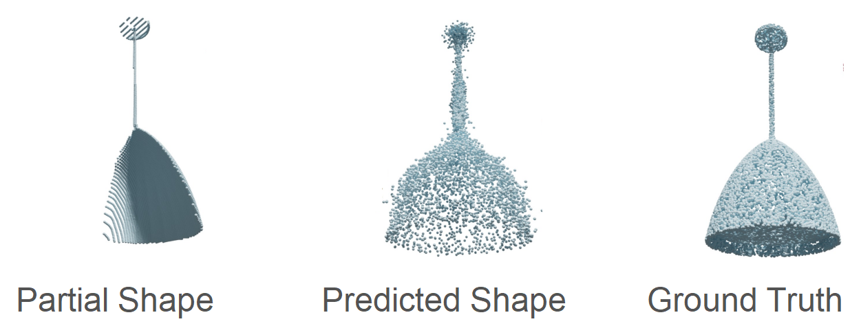
1. Smooth surfaces

The completed shape should have continuous and smooth surfaces, which is not the case in the predicted shape of the lamp below.

2. Fine details

We want to capture fine details of the object, such as an antenna on a car. In the image below the antenna is barely present in the input yet has not been modeled by the prediction.

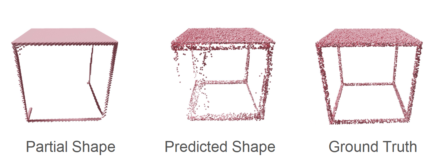
3. Locally even distribution of points

We want the points to be distributed evenly on the local parts of the object. When completing the shape of a table, we would expect the individual legs of the table below to have an even distribution of points, which should be considered in the prediction.

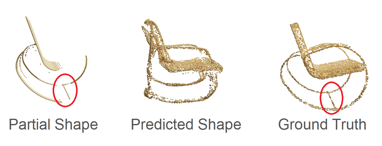
4. Preserve input structure

All parts of the object in partial input should be preserved in the completed shape. As we can see here, the little connector at the bottom of the chair has gone missing while producing the predicted shape.

Point Cloud Processing

PointNet

PointNet [2] is a seminal paper in point cloud processing because of its simple yet effective architecture. PointNet directly takes in a point cloud and produces a single feature vector through an auto-encoder and a final max-pool. Through feature transform layers, the network is also indifferent to the rotation of the point cloud and to the exact order of the points, which is an important feature to have since the points in a point cloud are unordered.

Point Cloud Generation

The task of point cloud generation is to take a compressed version of an input point cloud produced by an encoder (like in PointNet) and decode it back into a point cloud in 3D space. A naive way of doing that would be to directly predict each point in the point cloud. Altough simple, this approach cannot guarantee that we end up with smooth surfaces on the output shape. We’ll now look at some of the more sophisticated approaches for point cloud generation.

FoldingNet

FoldingNet [3] introduces a way of recovering the point cloud which resembles folding a piece of paper. FoldingNet samples points from a 2D grid and then deforms this 2D grid into the 3D shape in two passes. This type of decoder is referred to as a ‘morphing-based’ decoder and tends to produce shapes with continuous and smooth surfaces. The folding process can be seen in the image below.

AtlasNet

AtlastNet [4] uses a similar approach to FoldingNet. Instead of one 2D grid, multiple 2D grids are deformed into 3D surface elements, which then together build the final shape of the object. By using multiple grids, finer details of the shape can be captured.

We can see that deforming 2D grids into 3D surfaces is a promising approach to model smooth and continuous surfaces, which was one of our goals. Therefore we could view this kind of morphing-based decoder as our first puzzle piece needed to build a solid network for point cloud completion.

Point Completion Network (PCN)

Point Completion Network (PCN) [5] introduces the idea of modeling the rough shape of the object in an initial pass and then refining the details in a subsequent pass. This approach tends to produce more detailed shapes than if we had tried to predict the complete shape in one go. With the coarse-to-fine network we have the second puzzle piece for our point cloud completion network.

Contributions

Now that we have seen some methods used to generate point clouds we can turn to the Morphing and Sampling (MSN) paper. The papers makes four main contributions:

1. A novel two-stage approach for point cloud estimation.
2. The addition of an expansion penalty for surface elements.
3. A novel sampling algorithm for point clouds with evenly distributed results.
4. An Implementation of an Earth Mover’s Distance (EMD) approximation.

We will see later how each of these parts play a role in predicting completed object shapes which satisfy the four qualities presented in the last section. To recap, those are: smooth surfaces, fine details, a locally even distribution of points and preserving existing structure from the input.

Architecture

The architecture of the network in the MSN paper can be divided into four parts:

1. The Encoder and Morphing-based Decoder
2. Merging and Sampling
3. Refining
4. The Loss Function

 

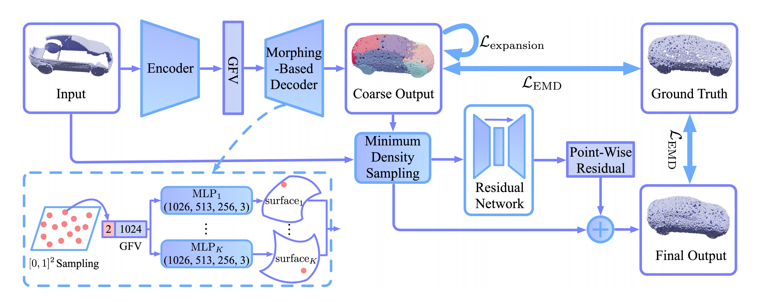
In the following section I’ll explain the individual parts of the network in more detail.

1. Encoder and Morphing-based Decoder

Generating the Coarse Shape

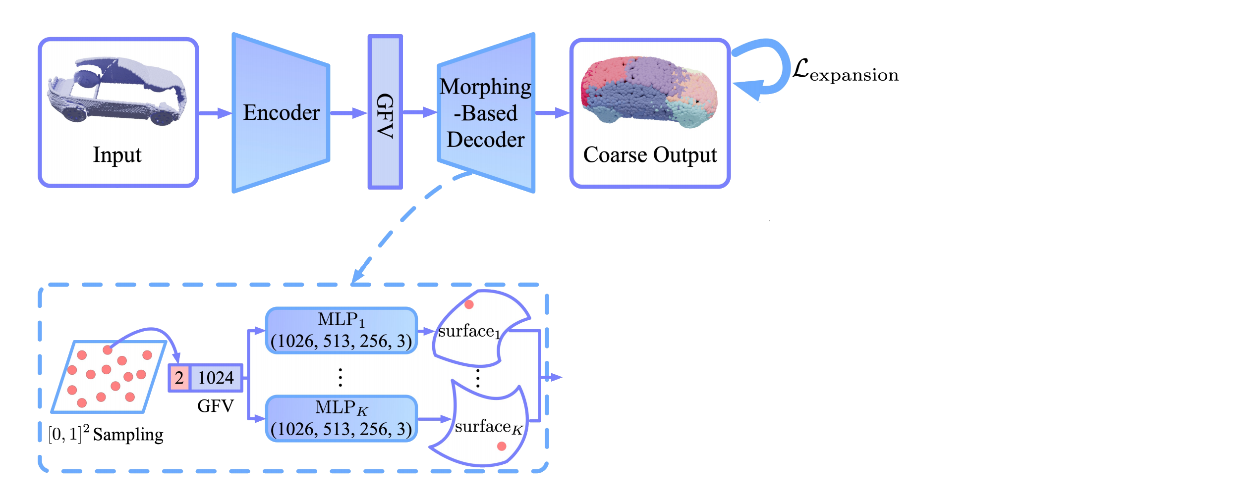
The encoder is based on PointNet and produces a single feature vector which encodes the input point cloud. In the decoder, we start with K 2D grids (K=16 in the paper). From those grids, n points (n=512 in the paper) are sampled and concatenated with the feature vector. The concatenated vectors are fed into K MLPs which deform them into K 3D surface elements as we have seen in the Point Completion Network. The surface elements together make up the coarse shape of the object with relatively smooth surfaces.

Morphing-based decoder to achieve smooth surfaces

In theory, the surface elements are not prohibited to overlap. To reduce overlap to a minimum, the authors introduce an ‘Expansion Penalty’ that is applied to the surface elements.

Expansion Penalty

The idea here is to encourage the surface elements to shrink to their respective center. This is done by construction a minimum spanning tree from the points of each surface element, with a total of K trees. A minimum spanning tree is a tree that connects all the vertices of a graph together without any cycles and with the minimum possible edge weight, where the edge weight here is the distance between two vertices. A loss function is applied to this spanning tree which penalizes long edges in the tree. To be exact, the function sums up for each spanning tree K all edges in the tree which are longer than the average edge in the tree l_i times a factor λ (a hyperparameter).

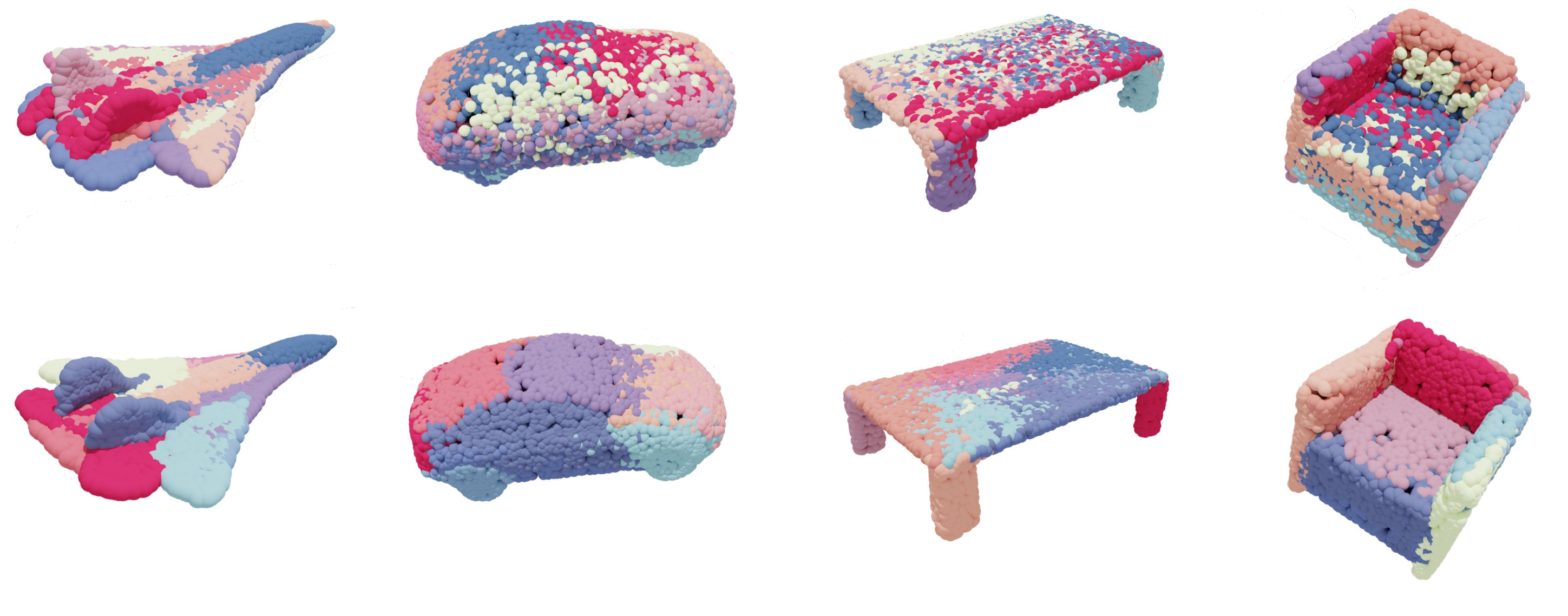
This way the vertices in the spanning tree are encouraged to migrate towards the middle vertex, which shrinks the surface elements towards its center. In the image below we can see the coarse output of the network on different objects, once without and once with the expansion penalty applied. Not only does the expansion penalty eliminate overlap, it also leads to the surface elements modeling different semantic parts of the object.

2. Merging and Sampling

Merging

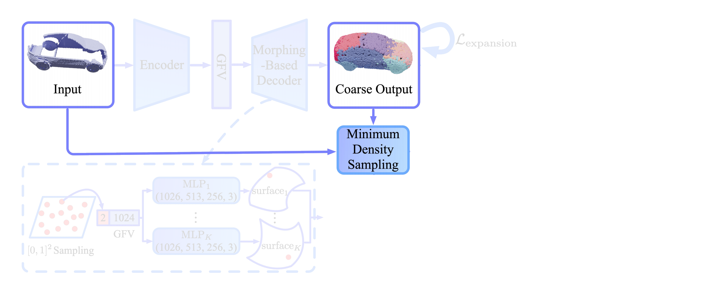
At this point we have modeled the coarse shape of the object with relatively smooth surfaces and a locally even distribution of points. That’s two out of the four goals checked so far. During the generation of the coarse shape, structures that are present in the input might have been dropped because the fixed-size surface elements can only model so much detail. To address this problem, the coarse point cloud is merged with the input point cloud. The two point clouds overlap in some areas (and not at all in other areas), therefore the merged point cloud likely has an uneven distribution of points. Through the merging operation we get to keep all structure from the input but the even distribution that was just there on the coarse point cloud is gone.

Merging with the input shape to preserve input structures

Sampling

To recover the even distribution of points, the authors propose to sample from the merged point cloud in a way that the sampled point cloud has an even distribution again. Unfortunately existing sampling algorithms such as Farthest Point Sampling (FPS) or Poisson Disk Sampling (PDS) preserve the unevenness in density and are not appropriate here.

The authors therefore come up with their own sampling algorithm called Minimum Density Sampling (MDS). In contrast to FPS, which samples the farthest point from the previously sampled points, MDS samples points in a way that the ‘density’ of the points in the sample is minimized. Density here is determined by the Gaussian-weighted distance of the point-to-sample to all previously sampled points. In the formula below, P_i-1 denotes the already sampled points and σ a hyperparameter which determines the size of the neighbourhood considered.

After sampling from the merged point clouds using MDS, the resulting point cloud now has a uniform distribution again.

3. Refining

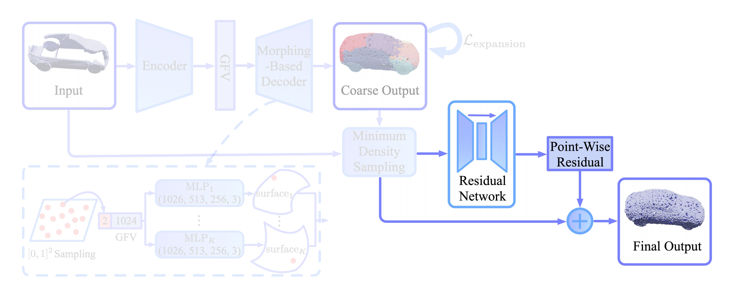
To generate fine-grained structures, the merged point cloud is fed into a residual network. The network consists of an encoder (based on PointNet) and a decoder which learns a refinement for each point that is then added point-by-point to the merged cloud.

Coarse-to-fine pass to model fine details of the object

At this stage we have generated the final output point cloud which represents the predicted complete shape of the object.

4. The Loss Function

To compare the predicted shape to the ground truth shape we need a metric that judges the similarity between the point clouds of the predicted and ground truth shape. Possible candidates for the distance metric are the Chamfer Distance (CD) and the Earth Mover’s Distance (EMD).

Chamfer Distance

The Chamfer Distance (CD) is a commonly used distance metric in point cloud completion tasks. Intuitively, for each point in one point cloud it computes the closest point in the second point cloud and then averages all the distances. The Chamfer Distance is straight-forward to calculate but when used as a loss function tends to produce shapes with blurry details and areas that are over-or underpopulated by points.

Earth Mover’s Distance

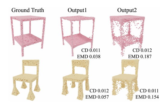
In contrast, the Earth Mover’s Distance tends to produce point clouds of higher quality. Intuitively, the Earth Mover’s Distance finds a bijection between the points of two point clouds and averages the distance between each pair of points. The bijection is chosen so that the average distance between corresponding points is minimized.

Earth Mover’s Distance for an even distribution of points

There are two downsides to the EMD. First, it requires the two point clouds to be of equal size. Second, finding the bijection is a challenging task of its own and the textbook implementation of such an algorithm requires memory in O(n²). With this kind of memory consumption, comparing point clouds of more than ~2000 points is not feasible.

To address the memory problem, the authors propose an algorithm that approximates the EMD with memory consumption of O(n), based on an algorithm from auction theory. In essence, the algorithm treats the points as persons and objects and auctions them off iteratively with the goal of reaching an economic equilibrium. In terms of computational cost, CD can be computed with O(n*log(n)) complexity, while the EMD approximation takes O(n²) computations. In the image below we can see that the EMD heavily penalizes point clouds with blurry surfaces, in contrast to the CD.

Final Loss Function

The final loss function is composed of the expansion loss of the coarse output as well as the EMD of the coarse and final output.

Putting it all together

Here we can see the structure of the complete network again. We have seen how the morphing-based decoder produces a coarse point cloud with smooth surfaces using surface elements and an expansion penalty. The coarse shape is then merged with the input shape to preserve existing input structures and sampled through Minimum Density Sampling to recover the uniform density of points. Following the sampling is a residual network which can model finer details of the object. The final output is then evaluated using EMD which warrants a locally even distribution of points.

Experiments

Evaluation Results

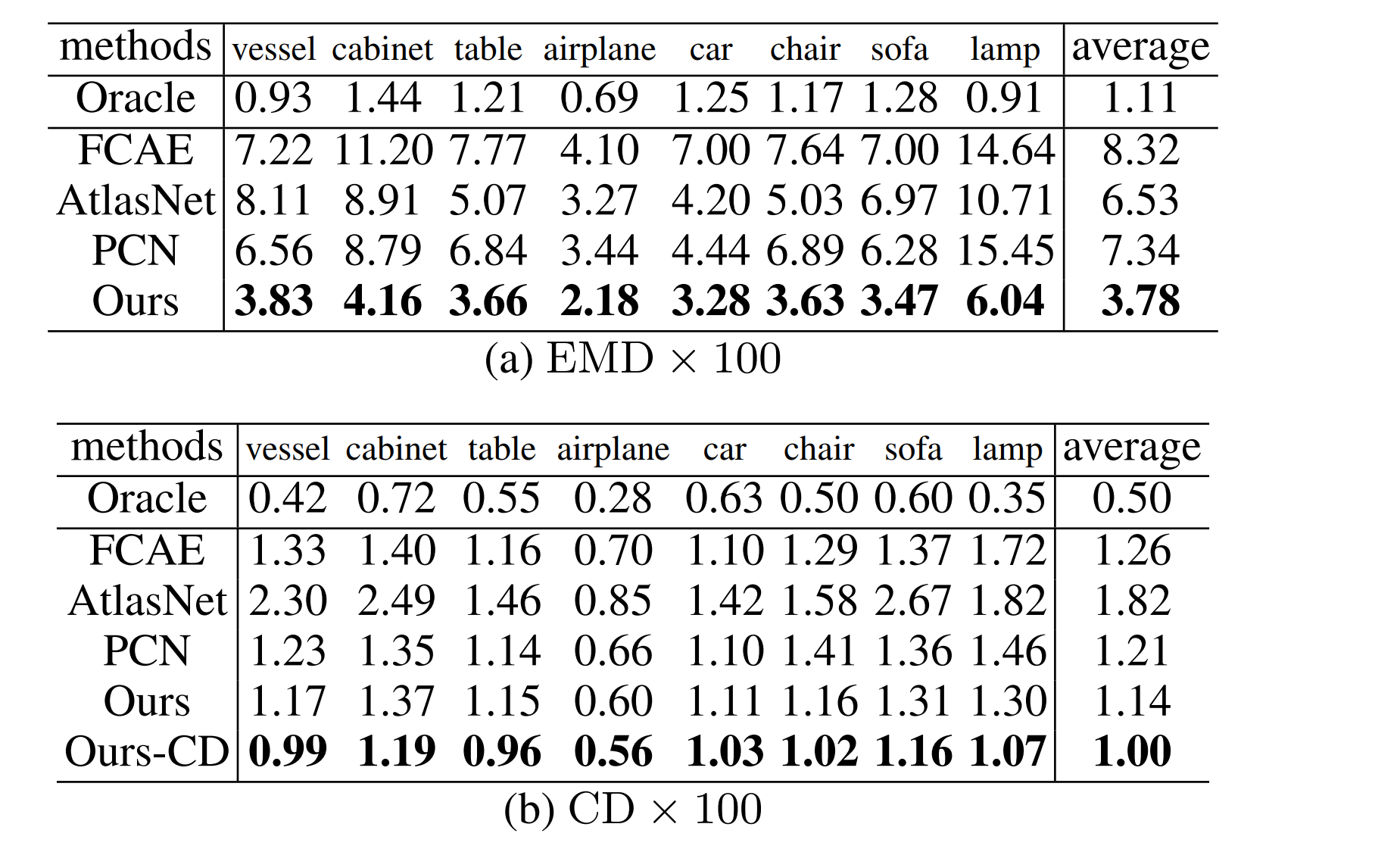
The network was evaluated on a subset of the ShapeNet dataset [5] wich includes eight classes of objects: table, chair, car, airplane, sofa, lamp, vessel, cabinet.

From ~30k objects in the dataset, 1.5million training samples were created by using varying camera poses to simulate different view angles.

While the network was trained on the EMD distance, it was evaluated both on the CD and EMD metrics. In both metrics, the network beats the state-of-the-art at the time of publishing the paper for each object class.

Qualitative results

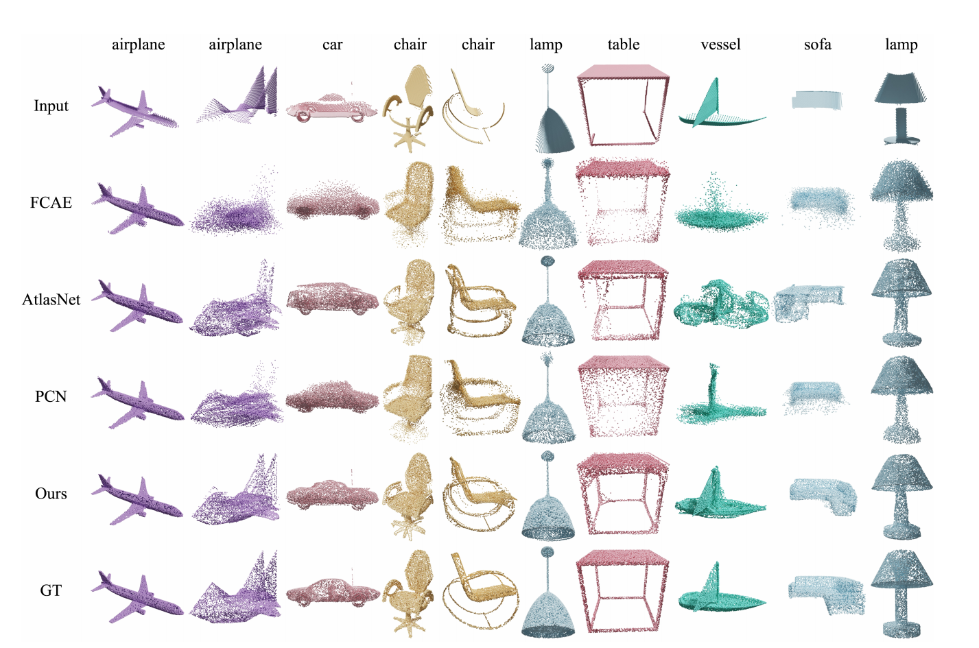
Below we can see qualitative results. Compared to the networks of previous papers, MSN tends to generate surfaces with less blur and finer details as well as getting the overall shape of the object right more often.

Ablation studies

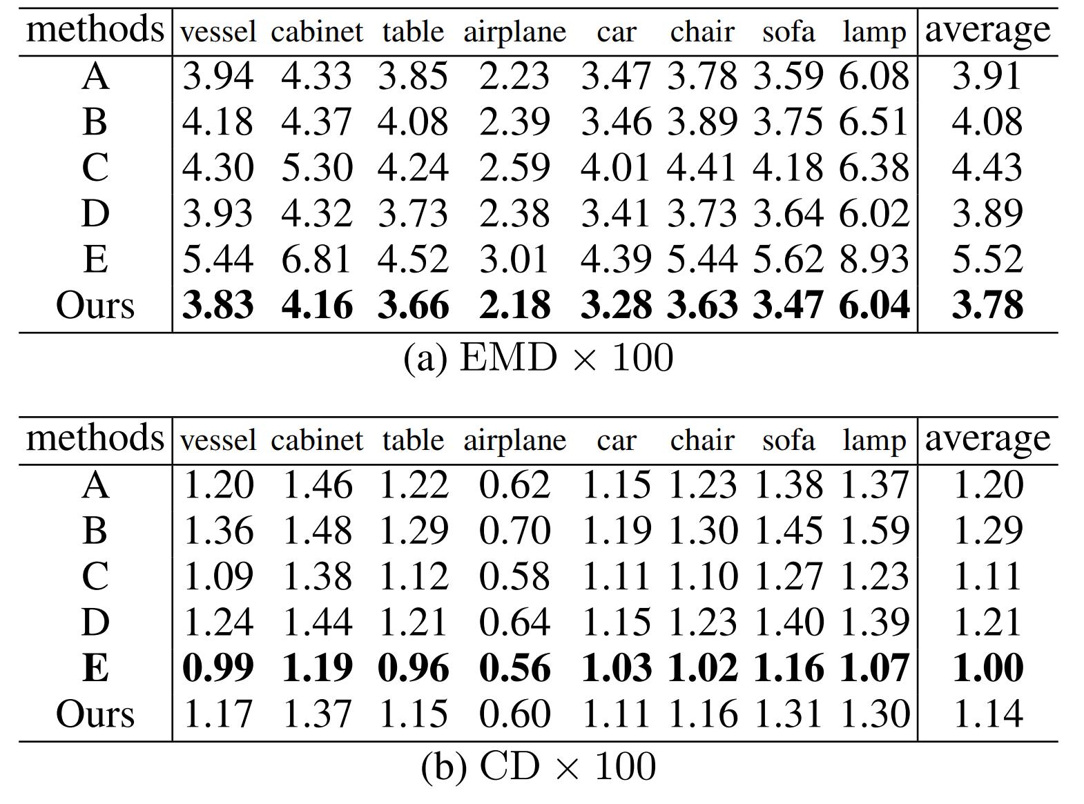
The authors have tested versions of the network where different parts were changed or omitted. These versions are:

A) Without expansion loss

B) Without merging and refining

C) Using FPS instead of MDS for the sampling

D) Without refining

The ablated versions of the network were, like in the evaluation, tested on both the Chamfer Distance and Earth Mover’s Distance. Versions A, B and C performed worse than the non-ablated version of the network on both distance metrics. For the sampling (C), the network evaluated on the Chamfer Distance provided better results with FPS than with the authors sampling algorithm (MDS). The explanation the authors give is that FPS results in a more uneven distribution of points, which is not as heavily penalized by CD than with EMD. On the other hand, FPS tends to preserve more points from the reliable input than MDS.

Conclusion

The authors have presented a novel way for point cloud completion where a coarse point cloud is generated in a first pass and then merged with the input point cloud and refined in a second pass. This approach generates smooth surfaces, preserves existing structure in the input and can generate fine-grained structures. The addition of an expansion penalty and a novel sampling algorithm as well as an approximation of the Earth Mover’s Distance ensure an even distribution of points. The network is able to generate realistic point clouds and achieves state-of-the-art results in point cloud completion.

My take on the paper

Method

The network was evaluated on both the native Earth Mover’s Distance as well as on the Chamfer Distance. The papers used to represent state-of-the-art for the evaluation are in my eyes a fair selection. On top of that, the authors have conducted extensive ablation studies. The network was evaluated on ShapeNet, which features dense point clouds. It would have also been interesting to see the performance on sparse data such as KITTI, albeit the authors state that the focus of the paper was on dense point cloud completion.

Architecture

In my eyes, the architecture is well thought-out an distinctly addresses the desired qualities of the output point cloud. Potential ways to improve the performance of the network could be to combine a folding-based decoder and a fully-connected decoder instead of only relying on a folding-based decoder. Also, explicitly trying to predict missing parts of the objects from the input point cloud could potentially improve the quality of the completed shapes.

General Assessment

The authors explain the network architecture concisely and in an easy to follow manner. What I find especially interesting about this paper is that the authors have presented solutions to existing problems, such as the approximation of the Earth Mover’s Distance as well as the Minimum density sampling algorithm. Earth Mover’s Distance, now that it has a feasible implementation, could improve the quality of future point cloud completion approaches and has been used to produce state-of-the-art results, for example in the Cloud Transformers network [8]. Although with a computational cost of O(n²) EMD is not a clear-cut choice over the CD.

Furthermore, point-cloud based methods are no longer the only successful approach to point cloud completion. Recent Voxel-based networks, such as GRNet [6], have overcome the drawbacks of voxelization and can deliver results that rival those of purely point-based networks.

References

Images not cited are taken from the MSN paper.

[1] Liu, M., Sheng, L., Yang, S., Shao, J., & Hu, S. M. (2020, April). Morphing and sampling network for dense point cloud completion. In Proceedings of the AAAI Conference on Artificial Intelligence (Vol. 34, No. 07, pp. 11596-11603).

[2] Qi, C. R., Su, H., Mo, K., & Guibas, L. J. (2017). Pointnet: Deep learning on point sets for 3d classification and segmentation. In Proceedings of the IEEE conference on computer vision and pattern recognition (pp. 652-660).

[3] Yang, Y., Feng, C., Shen, Y., & Tian, D. (2018). Foldingnet: Point cloud auto-encoder via deep grid deformation. In Proceedings of the IEEE Conference on Computer Vision and Pattern Recognition (pp. 206-215).

[4] Groueix, T., Fisher, M., Kim, V. G., Russell, B. C., & Aubry, M. (2018). A papier-mâché approach to learning 3d surface generation. In Proceedings of the IEEE conference on computer vision and pattern recognition (pp. 216-224).

[5] Yuan, W., Khot, T., Held, D., Mertz, C., & Hebert, M. (2018, September). Pcn: Point completion network. In 2018 International Conference on 3D Vision (3DV) (pp. 728-737). IEEE.

[6] ShapeNet: Chang, A. X., Funkhouser, T., Guibas, L., Hanrahan, P., Huang, Q., Li, Z., … & Yu, F. (2015). Shapenet: An information-rich 3d model repository. arXiv preprint arXiv:1512.03012.

[7] Xie, H., Yao, H., Zhou, S., Mao, J., Zhang, S., & Sun, W. (2020). GRNet: Gridding Residual Network for Dense Point Cloud Completion. arXiv preprint arXiv:2006.03761.

[8] Mazur, K., & Lempitsky, V. (2020). Cloud transformers. arXiv preprint arXiv:2007.11679.

[9] cs.cmu.edu/~wyuan1/pcn/images/shapenet.png, last accessed 12.01.2021

[10] Lim, I., Ibing, M., & Kobbelt, L. (2019, August). A Convolutional Decoder for Point Clouds using Adaptive Instance Normalization. In Computer Graphics Forum (Vol. 38, No. 5, pp. 99-108).